What Really Happens When You Run PCA on One-Hot Encoded Data?

A Visual Journey Reveals a Dangerous Data Science Artifact

Hi everyone,

In the world of data science, we have a standard toolkit. For categorical features, we often reach for One-Hot Encoding (OHE). For dimensionality reduction, we almost always start with Principal Component Analysis (PCA).

It seems natural to combine them. You one-hot encode your “city” or “product_category” feature, and then you run PCA on the resulting sparse matrix to reduce its dimensions. But what is PCA actually finding when you do this? The answer is both elegant and counter-intuitive, and understanding it is key to avoiding common interpretation pitfalls.

The Simple Case of Two Categories

Let's start with the simplest possible scenario: a single feature with only two categories, A and B. One-Hot Encoding transforms this into two columns. If the category is 'A', the vector is [1, 0]. If it's B, the vector is [0, 1].

Right away, we see a crucial fact: these two columns are perfectly redundant. Because the categories are mutually exclusive, the value of the B column is always 1 minus the value of the A column. This means that while we have two dimensions, there is only one degree of freedom.

This is the core idea of OHE, which we covered in detail last week. Feel free to check it out for a refresher:

What happens when we run PCA?

Figure 1: Visualizing PCA on a binary feature. Notice that PC1 captures 100% of the variance and perfectly connects the only two possible data points.

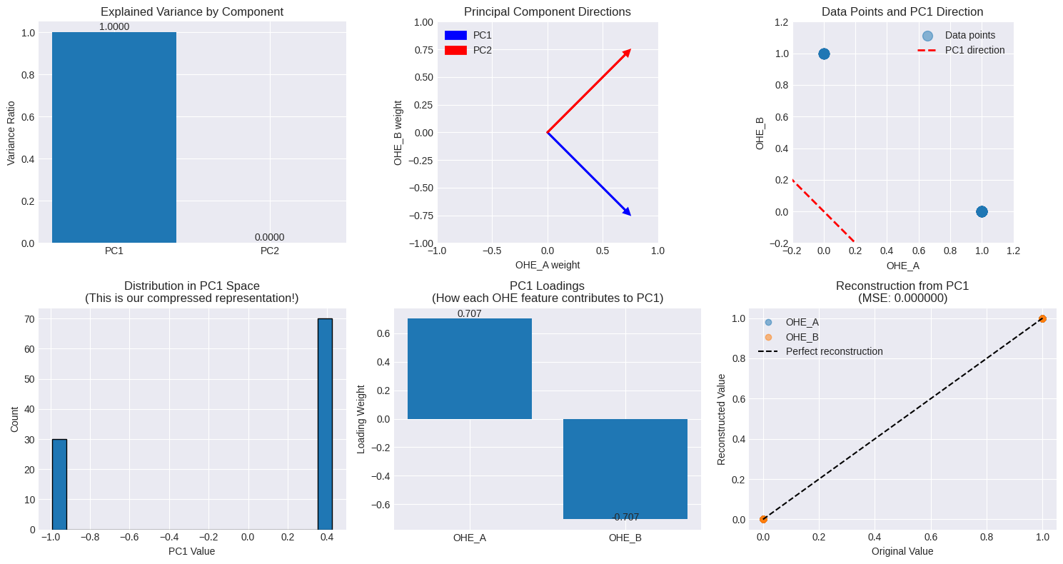
The plots above tell the whole story:

1. Explained Variance (Top-Left): The first principal component (PC1) captures 100% of the variance. The second (PC2) captures zero. PCA immediately identifies the redundancy.

2. Data Points & PC1 Direction (Top-Right): In the OHE space, our data can only exist at two points: (1, 0) and (0, 1). PCA finds the single straight line that connects these two points and explains all the variance. This line is the first principal component.

3. PC1 Loadings (Bottom-Middle): The loadings for PC1 are [0.707, -0.707]. This shows that PC1 represents a perfect opposition between feature A and feature B. Moving along this component means decreasing the A value and increasing the B value.

The takeaway is clear: in the simplest case, PCA doesn't discover a hidden pattern; it simply rediscovers the fundamental constraint of the encoding itself. No surprises here.

Beyond Two Categories: Probabilities vs. Eigenvalues

This is cool, but what happens with three categories? Or ten? As we increase the number of categories, k, a fascinating relationship emerges between the eigenvalues of the PCA and the underlying probabilities of the categories.

In short: the eigenvalues are not random. They are deeply connected to how frequently each category appears.

Figure 2: As the category probabilities move from uniform (top) to highly skewed (bottom), the corresponding eigenvalues from PCA mirror this change.

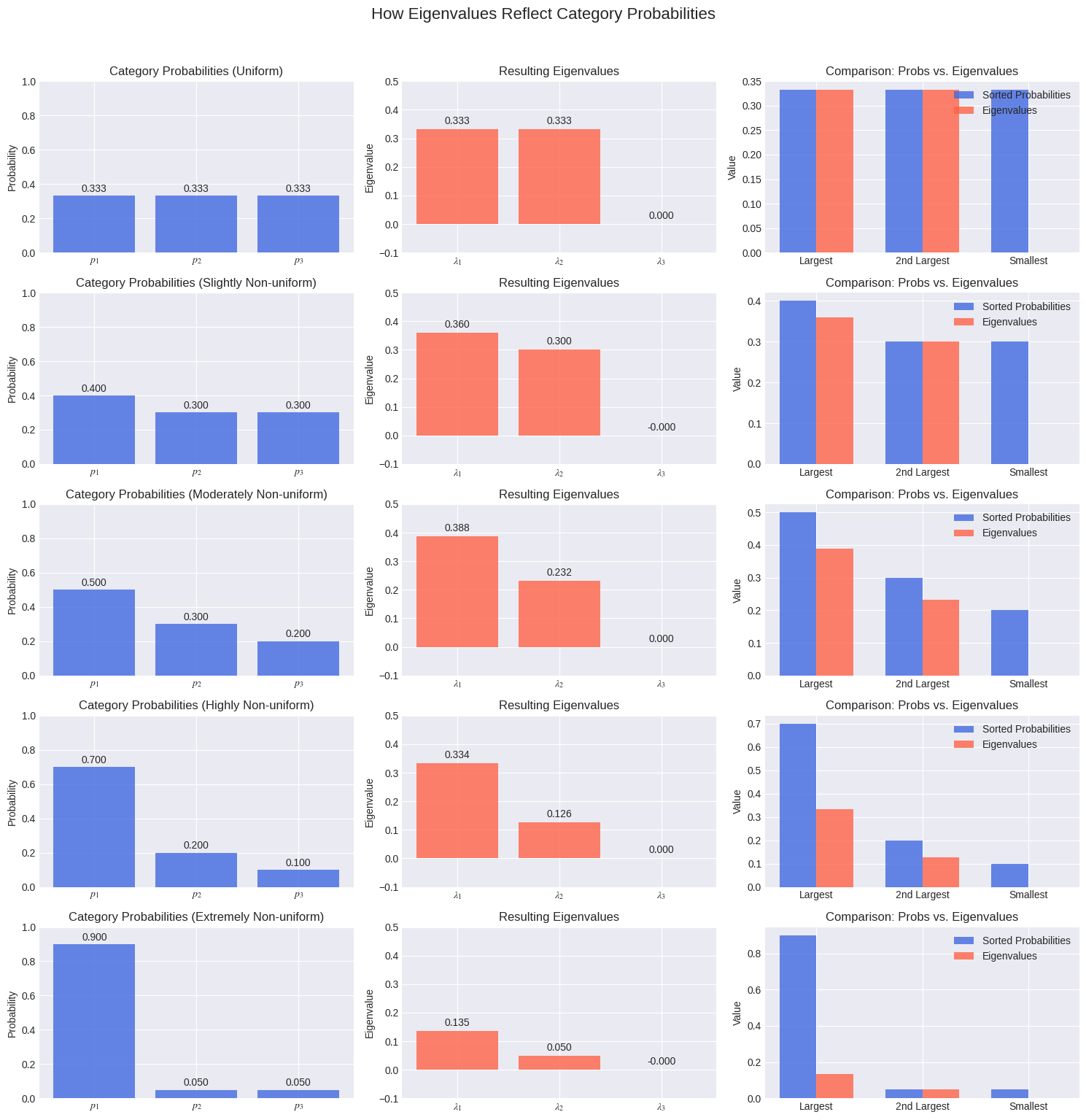
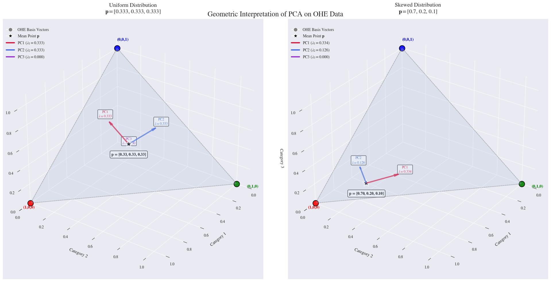
The plots above show this beautifully. For a 3-category feature:

• Uniform Probabilities: When each category has an equal probability (0.333), the two non-zero eigenvalues are also equal.

• Non-Uniform Probabilities: As soon as we make the probabilities unequal, the eigenvalues also become unequal, but they don't match the probabilities directly.

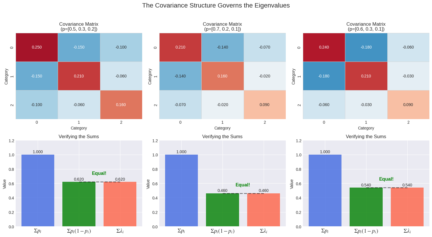
This relationship is governed by the covariance matrix of the OHE data. There are key properties that always hold:

1. Sum of eigenvalues = trace(Cov) = Σ pᵢ(1-pᵢ)

2. One eigenvalue is always zero due to the rank deficiency.

Figure 3: The covariance matrix of OHE data (top) and a confirmation that the sum of eigenvalues (red bar) always equals the sum of p(1-p) for the categories (green bar).

The Special Symmetry of the Uniform Distribution

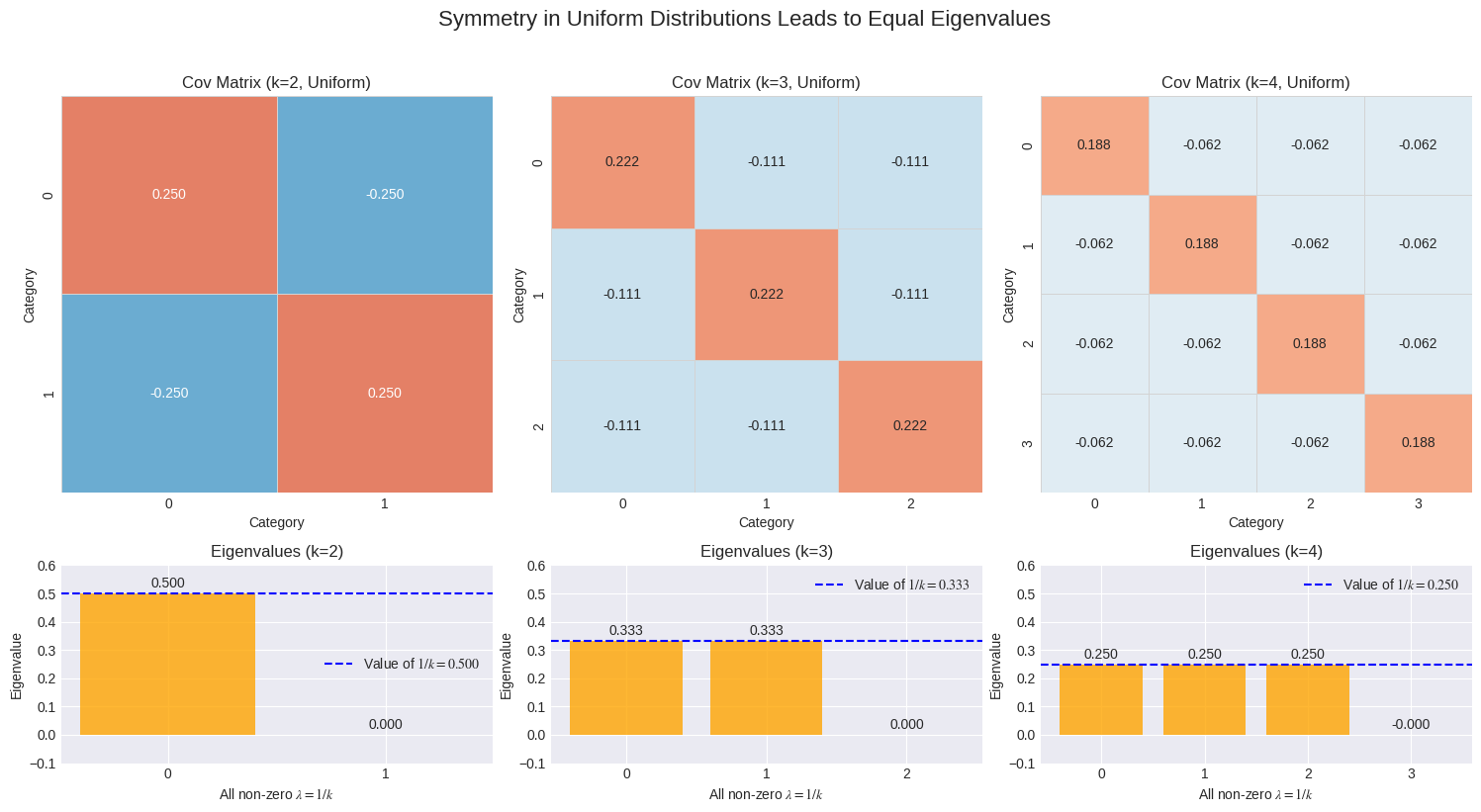
The case of a uniform distribution (where all categories are equally likely) is particularly elegant. This is the state of maximum entropy—maximum uncertainty. In this state, the covariance matrix becomes perfectly symmetric.

This symmetry leads to a clean, predictable result: for k categories, you get k-1 non-zero eigenvalues that are all exactly equal to 1/k.

Figure 4: For uniform distributions with k=2, 3, and 4, the non-zero eigenvalues are all identical, reflecting the perfect symmetry of the data.

A Quick Look at the Geometry

Geometrically, the one-hot encoded vectors form the vertices of a shape called a simplex. For three categories, our data lives at the corners of a triangle in 3D space: (1,0,0), (0,1,0), and (0,0,1).

All the data lies on the 2D plane that connects these three points. PCA simply finds the axes that best describe the spread of data on this plane, and the eigenvalues represent the amount of variance along those axes.

Figure 5: A geometric interpretation of PCA on OHE data. The principal components (colored arrows) describe the axes of variance on the 2D plane (the simplex) that contains the data.

What Happens When We Combine Features?

We've established how PCA behaves on a single OHE feature. But the real world is messy. What happens when we run PCA on a dataset with multiple OHE features?

The key thing to remember is that PCA is a global method. It doesn't know that some columns relate to one feature and others to another. It simply sees a point cloud and searches for the directions of maximum variance. This leads to a crucial question: which feature's structure will PCA prioritize?

This leads us to a powerful generalization, but with a critical nuance:

PCA prioritizes the directions of maximum variance one by one. The feature with the highest Total Variance Contribution will have a larger footprint on the PCA, but not necessarily the single largest eigenvalue.

The battle for dominance is fought component by component. A feature with its variance concentrated in one dimension can easily produce the single largest eigenvalue, even if its total variance is lower than another feature's. This is perfectly illustrated in the chart below.

Figure 6: A tale of two PCAs. On the left (Scenario A), the balanced binary feature (blue) has a total variance of 0.50, captured in a single eigenvalue of 0.50. The balanced 3-category feature (red) has a higher total variance of ~0.67, but this variance is split across two smaller eigenvalues (~0.34 and ~0.33). Therefore, the single most dominant principal component comes from the binary feature. On the right (Scenario B), the skewed 3-category feature's variance collapses to ~0.18, making the binary feature's 0.50 eigenvalue dominant by an even larger margin.

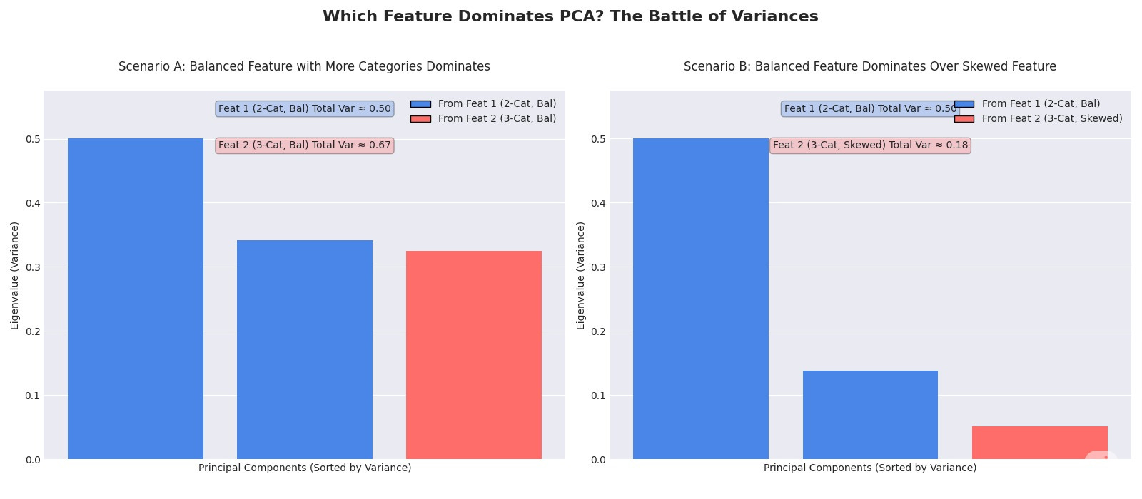
This effect isn't just limited to a battle between two and three categories. In fact, the dominance of the balanced, low-cardinality feature is a general rule. A balanced binary feature's single eigenvalue will always be 0.5. A balanced 4-category feature will produce three eigenvalues of 0.25 each. A balanced 10-category feature produces nine eigenvalues of 0.1 each. None of these individual components can ever overpower the one from the simple binary feature. This creates a predictable hierarchy where the most balanced features with the fewest categories will almost always produce the largest individual eigenvalues.

This leads us to the most critical takeaway of this entire analysis. Running PCA on a dataset of one-hot encoded features creates a predictable artifact. It systematically elevates features to the top of the importance list based on their statistical properties—balance and low cardinality—rather than their actual predictive power. Imagine you have a highly predictive but heavily skewed feature like zip_code (with thousands of categories) and a less predictive but perfectly balanced binary feature like gender. PCA will invariably flag the component representing gender as more important because it explains more variance. If you blindly select the top principal components for a downstream model, you risk building a model on features that are simply "loud" in the variance space, while ignoring the ones that are quiet but carry the real signal.

So, Is PCA on OHE a Good Idea?

After this journey, we can give a clear verdict. The answer is nuanced but direct:

PCA on OHE is a powerful exploratory tool but a dangerous automated step.

In fact, it really depends how do you use it. For Exploratory Data Analysis (EDA). Running PCA may quickly reveal some properties of your data.
However, as a pre-processing step for modeling, to reduce dimensionality, will be risky because PCA is selecting for variance, not predictive power. You are more likely to select for simple, balanced features than for complex, predictive ones.

---

This analysis shows that PCA on OHE is a technique with a surprising amount of hidden depth and potential pitfalls if used without care.

I'd love to hear your thoughts. Have you run into this artifact in your own work? What are your go-to methods for handling high-cardinality categorical features?

Thanks for following this deep dive, and I'll see you next week. See you next week!